Kinematics

Kinematics, in classical mechanics, study the description of the motion of points, bodies (objects), and groups of bodies without considering the forces that cause them to move. In mobile robotics, kinematics helps us to understand and quantify the constraints about the robot design, which implies restrictions in its movement. Also, we can draw the paths and trajectories that the robot can do. Here, the text focus on wheeled robots, which can only move in 2D space.

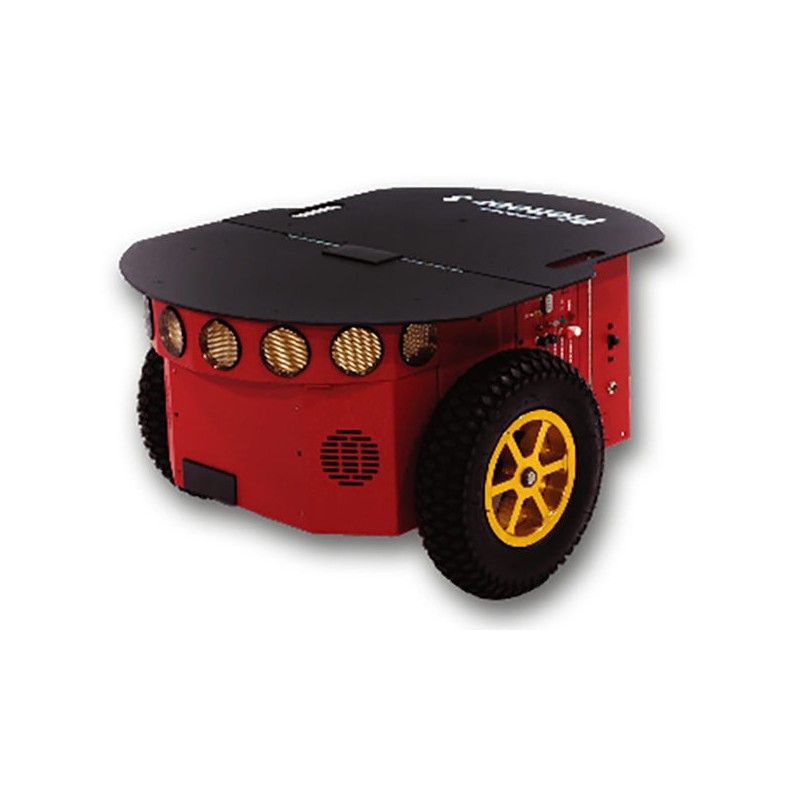
Pioneer P3-DX

Pioneer P3-AT

The P3-DX is a two-wheel-drive and P3-AT is a four-wheel-drive. The Omron Adept MobileRobots considers in its manual the P3-DX as a differential drive robot and the P3-AT as a skid/slip drive robot. For our sake, both are modeled as differential drive vehicles because the exact center of rotation in a skid/slip drive is unpredictable [1].

In order to represent the motion of a mobile robot, we must define the reference frames and determine their position. There are two essential frames to a robot if we consider the robot as a rigid body. They are the global reference frame, that is world fixed, and the local reference frame, which is robot fixed.

The global reference frame and the robot local reference frame. Figure from [1].

The figure shows a robot and its reference frames. Where the \(X_I\) and \(Y_I\) defines the global reference frame, also known as the inertial frame, and \(X_R\) and \(Y_R\) defines the local reference frame or the robot frame. The coordinates \(x\) and \(y\) represent the robot’s position in the global reference frame, point P, whereas \(\theta\) is the angular difference among the global and the local reference frames. Thus, we represent the robot’s pose as the vector with these three components.

\[\begin{split}\xi_I = \left[ \begin{array}{c} x \\ y \\ \theta \end{array} \right]\end{split}\]

Nota

We could still assume the robot as a rigid body free in the space, with 6 degrees of freedom, \([x, y, z, \phi, \psi, \theta]^T\). However, as the robot is moving subject to gravity, which keeps it confined to a euclidian plane, \(x\) and \(y\) describe the robot’s position, and \(\theta\) describes the orientation in the plane. The 2D space in which the robot lies is called the C-space [5], firstly formalized in [6], also called the configuration space. A configuration is a complete specification of the position of every point in the system. The space of all configurations is the C-space.

We can now utilize this definition to describe elements represented in the local frame in the global frame and vice-versa. For example, we can map the motion calculated in the global frame to motion in the robot’s local frame. Or, we can map obstacles sensed by the robot in terms of the global reference frame.

\[\begin{split}R(\theta) = \left[ \begin{array}{c} cos \theta & sin \theta & 0 \\ -sin \theta & cos \theta & 0 \\ 0 & 0 & 1 \end{array} \right]\end{split}\]

The orthogonal rotation matrix does the map between these frames as a function of the robot’s current pose.

\[\dot{\xi_R} = R(\theta) \dot{\xi_I}\]

Nota

It does not make sense to talk about the robot’s pose in the local frame. Because, the point P, the origin of the coordinates, moves around with the robot. So, the robot’s pose in the local frame is, always, \(\xi_R = [0, 0, 0]^T\). That is why the relationship is between the derivative of the pose in the frames.

Wheels and its constraints

«Wheeled Mobile Robots (WMR) constitute a class of mechanical systems characterized by kinematics constraints that are not integrable and cannot, therefore, be eliminated from the model equations» [2]. If we want to study and describe a robot motion, we also must specify which are the hypotheses and constraints of the wheels. There are three essential hypotheses about the kinematics model of the wheeled robot during the motion; they are:

• Each wheel remain perpendicular about its plane;
• There is only one contact point between plane and wheel;
• There is only rolling without slipping;

And two constraints:

• About rolling: the motion component along the wheel plane is equal to the rotation velocity of the wheel;
• About slipping: the motion component along the orthogonal direction is equal to zero;

Some authors may call these constraints as «the pure rolling and rotation condition».

Differential Drive Model

Now we delve into modeling of a differential drive kinematic. Dudek et al. say that the differential drive consists of two wheels mounted in the same axis with separated motors [3]. Each wheel contributes to the robot motion, so to fully describe the robot motion, we must compute each contribution.

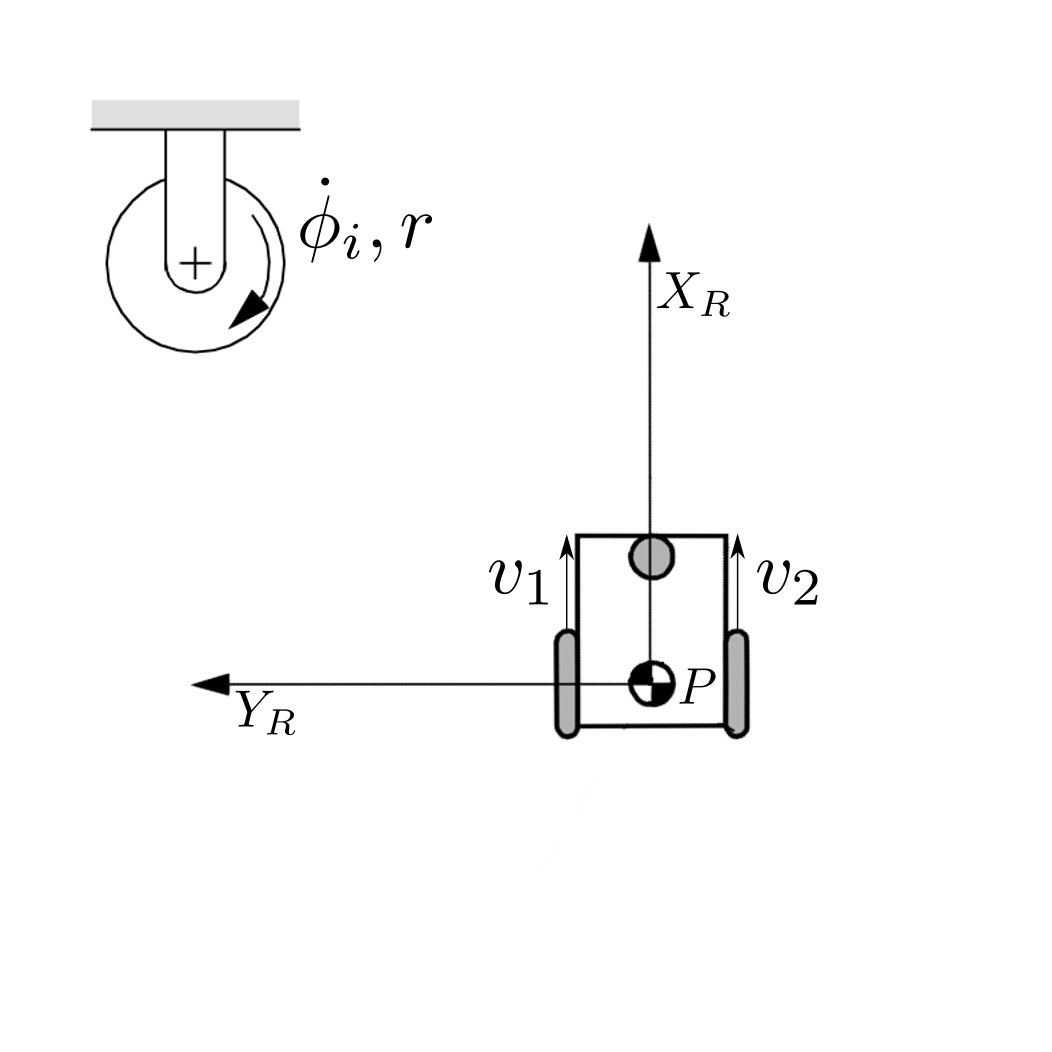
Wheel velocities and the robot frame.

The image shows the robot, the wheel velocities, and the local frame. \(\dot{\phi}_1\) and \(\dot{\phi}_2\) is the spin speed of the left wheel and right wheel. \(r\) is the wheel radius, while the distance between the two wheels is \(l\). While \(v_1\) is the left wheel velocity along the ground and \(v_2\) the right wheel velocity. As the wheels contribute independently to the robot motion, we can analyze each contribution separately.

\[\begin{split}\begin{array}{c} v_i = \frac{\dot{\phi}_i r}{2} \\ \omega_i = \frac{\dot{\phi}_i r}{2 l} \\ \text{where } i = \{1, 2\} \end{array}\end{split}\]

Point \(P\) is halfway between the two wheels, so each wheel contributes with half of the linear speed of the robot in the direction of \(X_R\). Each wheel also adds a new component to the angular speed of the robot. \(v_1\) moves the robot clockwise around point \(P\) while \(v_2\) moves it counter-clockwise. That is why they differ in their sign. And, using the equation which relates the angular speed of disk with its linear speed, we have the above equations.

Using the superposition theorem, we have the equations for the linear velocity in the direction of \(X_R\) and the angular velocity in the direction of \(Z_R\):

\[\begin{split}\begin{array}{c} v & = & v_1 + v_2 \\ \omega & = & -\omega_1 + \omega_2 \end{array}\end{split}\]

In the local frame, we have the following kinematic equation:

\[\begin{split}\dot{\xi_R} & = & \left[ \begin{array}{c} \frac{r}{2} & \frac{r}{2} \\ 0 & 0 \\ -\frac{r}{2 l} & \frac{r}{2 l} \end{array} \right] \left[ \begin{array}{c} \dot{\phi}_1 \\ \dot{\phi}_2 \end{array} \right]\end{split}\]

Nota

In the robot frame, there is no velocity in the direction of \(Y_R\). Because we assumed the pure rolling and rotation condition. And yet he can reach any point in the global frame.

Forward Kinematics

The forward kinematics problem tries to solve the problem when we have the control inputs, and we must know where the robot goes in the global frame. As we have seen, to solve this question, we should know five parameters of the robot — two parameters about the robot geometry, \(l\) and \(r\), the current robot orientation, \(\theta\), and, at least, the two inputs, \(\dot{\phi}_1\) and \(\dot{\phi}_2\).

\[\begin{split}\dot{\xi_I} = \left[ \begin{array}{c} \dot{x} \\ \dot{y} \\ \dot{\theta} \end{array} \right] = f(l, r, \theta, \dot{\phi_1}, \dot{\phi_2})\end{split}\]

\(f\) is the function that solves the forward kinematics problem. To map between the parameter vector, \(\{l, r, \theta, \phi_1, \phi_2\}\), and the state of the robot in the inertial frame. We should use the matrix, which links the spin speed and the derivative of the robot state in the local frame. Then, we can transform the robot velocities in the local frame to the global frame utilizing the inverse of the rotation matrix.

\[\begin{split}\begin{array}{c} R(\theta)^{-1} = \left[ \begin{array}{c} cos \theta &-sin \theta & 0 \\ sin \theta & cos \theta & 0 \\ 0 & 0 & 1 \end{array} \right], & \dot{\xi_I} = R(\theta)^{-1} \dot{\xi_R}, & \dot{\xi_R} = \left[ \begin{array}{c} \frac{r}{2} & \frac{r}{2} \\ 0 & 0 \\ -\frac{r}{2 l} & \frac{r}{2 l} \end{array} \right] \left[ \begin{array}{c} \dot{\phi}_1 \\ \dot{\phi}_2 \end{array} \right] \end{array}\end{split}\]

\[\begin{split}\dot{\xi_I} & = & R(\theta)^{-1} \left[ \begin{array}{c} \frac{r}{2} & \frac{r}{2} \\ 0 & 0 \\ -\frac{r}{2 l} & \frac{r}{2 l} \end{array} \right] \left[ \begin{array}{c} \dot{\phi}_1 \\ \dot{\phi}_2 \end{array} \right]\end{split}\]

Then,

\[\begin{split}f(l, r, \theta, \dot{\phi_1}, \dot{\phi_2}) & = & \left[ \begin{array}{c} cos \theta &-sin \theta & 0 \\ sin \theta & cos \theta & 0 \\ 0 & 0 & 1 \end{array} \right] \left[ \begin{array}{c} \frac{r}{2} & \frac{r}{2} \\ 0 & 0 \\ -\frac{r}{2 l} & \frac{r}{2 l} \end{array} \right] \left[ \begin{array}{c} \dot{\phi}_1 \\ \dot{\phi}_2 \end{array} \right]\end{split}\]

\[\begin{split}f(l, r, \theta, \dot{\phi_1}, \dot{\phi_2}) & = & \left[ \begin{array}{c} \frac{r cos \theta}{2} & \frac{r cos \theta}{2} \\ \frac{r sin \theta}{2} & \frac{r sin \theta}{2} \\ -\frac{r}{2 l} & \frac{r}{2 l} \end{array} \right] \left[ \begin{array}{c} \dot{\phi}_1 \\ \dot{\phi}_2 \end{array} \right]\end{split}\]

Or

\[\begin{split}\dot{\xi_I} & = & \left[ \begin{array}{c} \frac{r cos \theta}{2} & \frac{r cos \theta}{2} \\ \frac{r sin \theta}{2} & \frac{r sin \theta}{2} \\ -\frac{r}{2 l} & \frac{r}{2 l} \end{array} \right] \left[ \begin{array}{c} \dot{\phi}_1 \\ \dot{\phi}_2 \end{array} \right]\end{split}\]

Nota

The matrix which maps spin speed to the robot velocities is commonly known as Jacobian Matrix. «The Jacobian maps configuration velocities to workspace velocities» [5].

Well, we know the relationship between spin speeds and robot velocities, but what about the robot pose in the global frame?

\[\begin{split}\xi_I = \int_{0}^{t} \left[ \begin{array}{c} \frac{r cos \theta}{2} & \frac{r cos \theta}{2} \\ \frac{r sin \theta}{2} & \frac{r sin \theta}{2} \\ -\frac{r}{2 l} & \frac{r}{2 l} \end{array} \right] \left[ \begin{array}{c} \dot{\phi}_1 \\ \dot{\phi}_2 \end{array} \right] dt\end{split}\]

Or

\[\begin{split}\begin{cases} x(t) = \frac{r}{2} \int_{0}^{t} (\dot{\phi_1}(t) + \dot{\phi_2}(t)) cos (\theta(t)) dt \\ y(t) = \frac{r}{2} \int_{0}^{t} (\dot{\phi_1}(t) + \dot{\phi_2}(t)) sin (\theta(t)) dt \\ \theta(t) = \frac{r}{2 l} \int_{0}^{t} (\dot{\phi_2}(t) - \dot{\phi_1}(t)) dt \end{cases}\end{split}\]

Inverse Kinematics

The inverse kinematics problem is the opposite of the forward problem. The problem aims to solve the following question: «Given the desired pose, which are the controls needed to reach the desired pose?». We already know the relationship between the velocity and

\[\begin{split}\left[ \begin{array}{c} \dot{\phi_1} \\ \dot{\phi_2}\end{array} \right] = g(\dot{\xi_I})\end{split}\]

The function \(g\) is the mathematical inverse of the function \(f\).

\[\begin{split}g = f^{-1} = \left[ \begin{array}{c} \frac{r cos \theta}{2} & \frac{r cos \theta}{2} \\ \frac{r sin \theta}{2} & \frac{r sin \theta}{2} \\ -\frac{r}{2 l} & \frac{r}{2 l} \end{array} \right]^{-1}\end{split}\]

As we can see, the matrix which represents the function \(f\) is not invertible. The forward kinematics is an easy problem because we have one and only one solution. Nevertheless, the inverse kinematics is often not analytically solvable; commonly, we have more than one solution or none. However, we can try to solve the problem, limiting the possibles solutions like \(\dot{\phi}_1 = \dot{\phi}_2\) or \(\dot{\phi}_1 = -\dot{\phi}_2\).

Straight Line

If we limit the solution to \(\dot{\phi}_1 = \dot{\phi}_2 = \dot{\phi}\), with \(\dot{\phi} > 0\), the robot should move along a straight line. Then, the robot motion simplifies to:

\[\begin{split}\xi_I = \left[ \begin{array}{c} x' \\ y' \\ \theta' \end{array} \right] = \left[ \begin{array}{c} x + v cos (\theta) \delta t \\ y + v sin (\theta) \delta t \\ \theta \end{array} \right]\end{split}\]

Rotaion in place

Similarly, if we limit the solution to \(-\dot{\phi}_1 = \dot{\phi}_2\), with \(\dot{\phi}_2 > 0\), the robot should rotate in the place around the point P.

\[\begin{split}\xi_I = \left[ \begin{array}{c} x' \\ y' \\ \theta' \end{array} \right] = \left[ \begin{array}{c} x \\ y \\ \theta + \frac{2 v}{l} \delta t \end{array} \right]\end{split}\]

Motion Composition

If we would like to drive the robot from any pose to some other pose in the global frame, we can decompose the motion in two rotations in place and one translation along a straight line. The robot can turn in the place aligning its orientation aiming the goal position, \((x_d,y_d)\), then move forward to the goal position, and then turn in the place again to reach the goal orientation, \(\theta_d\).

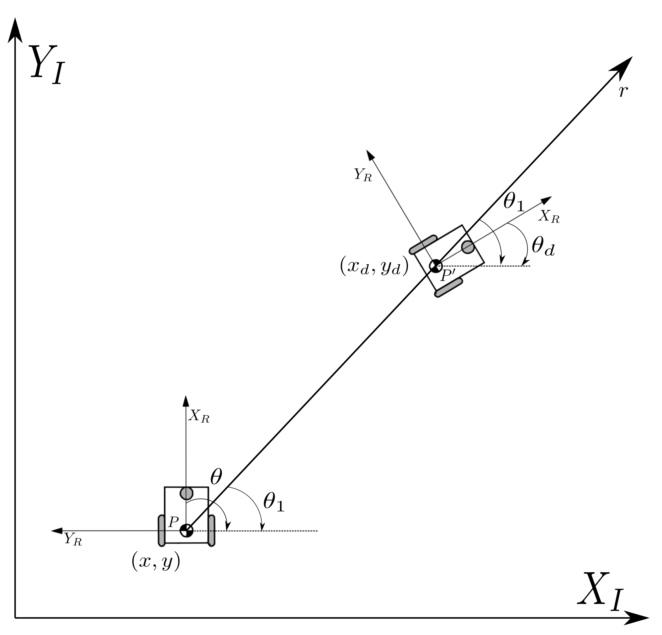
A robot is moving around with the proposed motion framework.

The image above tries to illustrate the proposed motion. The robot starts with the \(\xi_I = [ x, y, \theta ]^T\). Then it spun around the point \(P\) and aim the desired position \(P' = (x_d,y_d)\) reaching the pose \(\xi'_I = [ x, y, \theta_1 ]^T\). To reach the position, it moves forward to \(P' = (x_d,y_d)\) and reaches \(\xi''_I = [ x_d, y_d, \theta_1 ]^T\). And then the robot spun again to from \(\theta_1\) to \(\theta_d\). The final robot state should be \(\xi'''_I = [ x_d, y_d, \theta_d ]^T\).

The Unicycle Model

So far, we saw the kinematics of a two-wheeled robot. But now we talk about a more general and simple model. The previous model tells us how a robot with two wheels can reach a specific pose in the world, acting in the wheel speeds. But, we do not care about how the wheel is turning; we care about the pose of the robot. The unicycle model represents a robot with only one wheel. If the wheel complies with our pure rotation and rolling condition, the wheel has two control inputs, the linear velocity, \(v\), in the axis \(X_R\) and the angular velocity, \(\omega\), around \(Z_R\). So, the kinematics of a unicycle robot described in the inertial frame \(\{ X_I , Y_I , θ \}\) is given by

\[\begin{split}\left[ \begin{array}{c} \dot{x} \\ \dot{y} \\ \dot{\theta} \end{array} \right] & = & \left[ \begin{array}{c} v \cos \theta \\ v \sin \theta \\ \omega \end{array} \right] & = & \left[ \begin{array}{c} \cos \theta & 0 \\ \sin \theta & 0 \\ 0 & 1 \end{array} \right] \left[ \begin{array}{c} v \\ \omega \end{array} \right]\end{split}\]

Where \(x\), \(y\) and \(\theta\) are the coordinates of the robot in the global frame and \(u = (v, \omega)\) is the control vector.

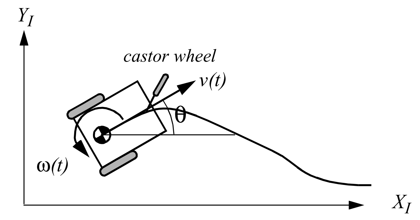
A differential-drive robot in its global reference frame. Figure from [1].

Commercial robots usually provide an interface to translate from a desired unicycle control input to desired wheel velocities. And a lower level dedicated microcontroller, which aims to control the wheel velocities.

Notes on Control

So, we should be able to build a system or software capable of, using the maths showed, move a robot to any reachable goal. The control theory is the branch of maths dedicated to this problem. A control system sends inputs to the system and leads the variables of the system to the desired goal. Our system is a mobile robot. And, using the previous equations, the inputs are the spin speed of each wheel, and the output is the pose of the robot.

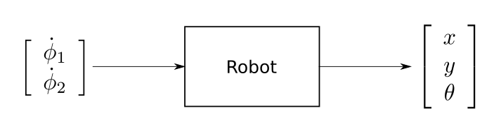
A controller should give the system the inputs necessary to perform the desired action. As in the image below:

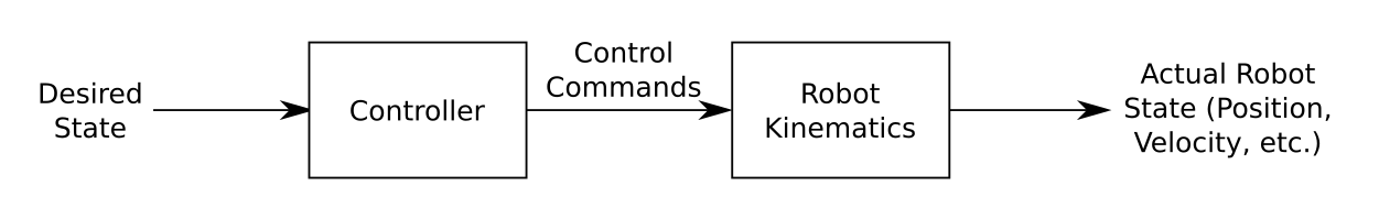
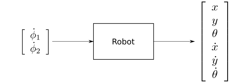
If we see the controller and the robot as a single system, we can have another system with the desired state as input and the robot state as output. Then we can build a new controller which deals with choosing the desired state. In the same manner, if we would like to control the velocities of the robot and not only the pose, to be able to control how the robot moves. We can add the velocities to the robot state vector and control them with the equations related.

Nota

A differential drive robot has a major problem which is… Feng et al. [4] develops in 1993 a motion controller which…

[1]	(1, 2, 3) Roland Siegwart and Illah R. Nourbakhsh. 2004. Introduction to Autonomous Mobile Robots. Bradford Company, USA.

[2]	Campion, G. Bastin and B. Dandrea-Novel, «Structural properties and classification of kinematic and dynamic models of wheeled mobile robots,» in IEEE Transactions on Robotics and Automation, vol. 12, no. 1, pp. 47-62, Feb. 1996.

[3]	Gregory Dudek and Michael Jenkin. 2010. Computational Principles of Mobile Robotics (2nd. ed.). Cambridge University Press, USA.

[4]	Feng, Y. Koren and J. Borenstein, «Cross-coupling motion controller for mobile robots,» in IEEE Control Systems Magazine, vol. 13, no. 6, pp. 35-43, Dec. 1993.

[5]	(1, 2) Choset, K. M. Lynch, S. Hutchinson, G. Kantor, W. Burgard, L. E. Kavraki and S. Thrun, «Principles of Robot Motion: Theory, Algorithms, and Implementations,» MIT Press, Boston, 2005.

[6]	Lozano-Perez, «Spatial Planning: A Configuration Space Approach,» in IEEE Transactions on Computers, vol. C-32, no. 2, pp. 108-120, Feb. 1983.